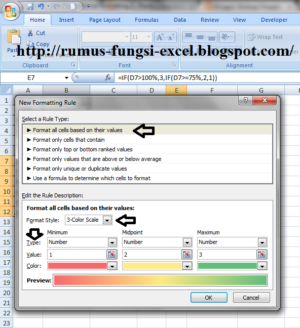
Cara Menggunakan Conditional Formatting Dengan Rumus If Perhitungan Soal
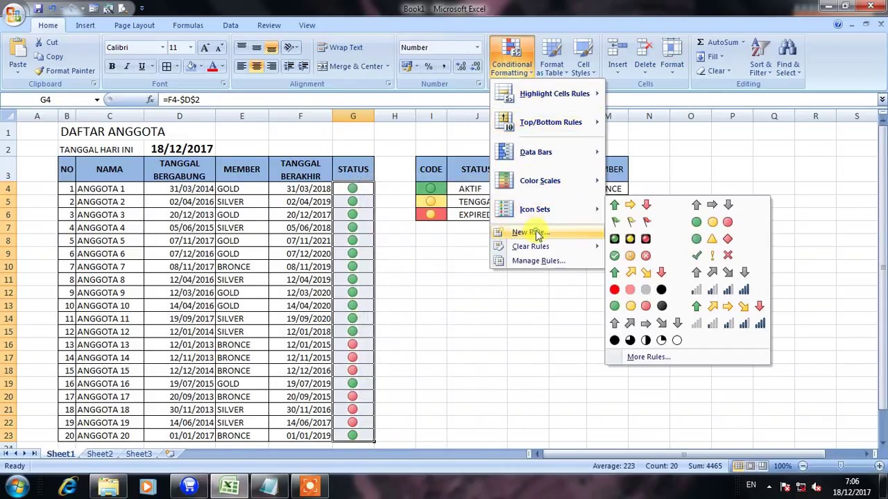
Select the range of cells where you want to apply the icons. Click Conditional Formatting > Icon Sets > More Rules. In the New Formatting Rule dialog box, select the desired icons. From the Type dropdown box, select Percentage, Number of Formula, and type the corresponding values in the Value boxes. Finally, click OK.

Cara Menggunakan Conditional Formatting YouTube
2. Create a conditional formatting rule, and select the Formula option. 3. Enter a formula that returns TRUE or FALSE. 4. Set formatting options and save the rule. The ISODD function only returns TRUE for odd numbers, triggering the rule: Video: How to apply conditional formatting with a formula.
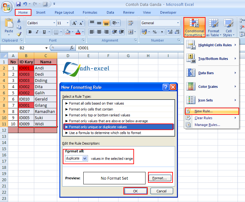
Conditional Formatting, Cara Mencari Data Ganda/Duplikat Dalam Excel panduan bisnis online
Video ini menjelaskan cara memberikan warna otomatis di 1 Baris dengan menggunakan Conditional Formatting. File latihan bisa didownload gratis di sini: https.

cara memanfaatkan conditional formatting di Microsoft Office Excel. YouTube
Select the names dataset (excluding the headers) Click on "Format" > "Conditional formatting". Select the " Add another rule " option. 4. Ensure the range (where you'll highlight the duplicates) is correct. If it isn't, change it from the "Apply to range" section. Click on "Format cells if" > "Custom formula is".
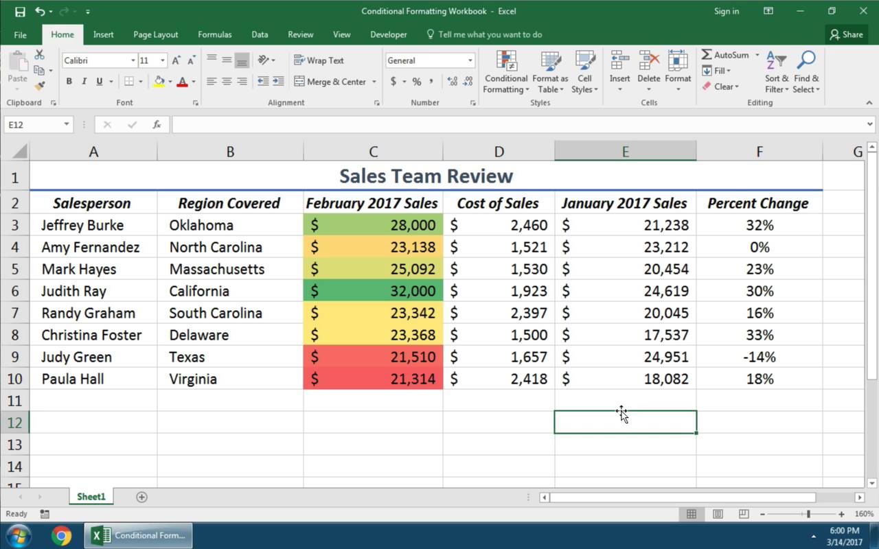
How to Use Conditional Formatting in Microsoft Excel Envato Tuts+
To accomplish this, the steps are: Click Conditional formatting > Highlight Cells Rules > Greater Than…. In the dialog box that pops up, place the cursor in the text box on the left (or click the Collapse Dialog icon), and select cell D2. When done, click OK.

Excel Conditional Formatting De Linha Baseada Em Texto Da Célula La Texto
Copy the selected cells by pressing the Ctrl + C. Select the range where the Conditional Formatting is to be pasted. Right-click the selection and point to Paste Special from Paste Options in the opened context menu. Under Other Paste Options, click on the Formatting button.
Cara Membuat Conditional Formatting Di Excel 2010 Text Warga.Co.Id
On the Home tab, in the Styles group, click the arrow next to Conditional Formatting, and then click Manage Rules. The Conditional Formatting Rules Manager dialog box appears. The conditional formatting rules for the current selection are displayed, including the rule type, the format, the range of cells the rule applies to, and the Stop If.

Cara Membuat Timeline Pekerjaan di Excel Menggunakan Conditional Formatting YouTube
Under the Home tab, click on the Conditional Formatting button (in the Styles group). This will display a drop-down menu with different conditional formatting options. Select ' New Rule'. This will open the ' New Formatting Rule ' dialog box. From the options under ' Select a Rule Typ e', click on the option ' Use a formula to.

Cara Mewarnai Progress Bar di Sel Excel dengan Conditional Formatting YouTube
Take your Excel skills to the next level and use a formula to determine which cells to format. Formulas that apply conditional formatting must evaluate to TRUE or FALSE. 1. Select the range A1:E5. 2. On the Home tab, in the Styles group, click Conditional Formatting. 3. Click New Rule. 4. Select 'Use a formula to determine which cells to format.

Cara membuat conditional formatting di spreadsheet
Mirip dengan grafik dan sparklines, format kondisional menyediakan cara lain untuk memvisualisasikan data dan membuat lembar kerja lebih mudah untuk dipahami. Opsional: Unduhlah praktek workbook kita.. Terapkan Conditional Formatting sehingga akan meng-Highlights Sel yang mengandung nilai-nilai Kurang Dari 70 dengan mengisinya warna merah.

🔴TIPS EXCEL Cara Membuat CONDITIONAL FORMATTING, menggunakan rumus IF dan MATCH YouTube
Kemudian, buka menu Format dan pilih Conditional Formatting. Buka menu Format > Conditional Formatting di Google Sheets untuk mulai menambahkan aturan tertentu. Di sisi kanan Sheets, Anda akan melihat panel terbuka yang berjudul Conditional Format Rules. Panel ini akan mengarahkan bagaimana menerapkan format bersyarat ke sel di Google Sheets.

Cara Conditional Formating di Google Sheets (Memberi Warna Pada Huruf dan Angka Tertentu) YouTube
Let's select the entire Headquarters column and click on Format tab and select Conditional formatting. By default, it will apply conditional formatting on the complete column. Then in the Format rules under Format cells if. click on the drop-down menu, and select Text contains which will then let you put the text.

Cara Menggunakan Conditional Formatting Excel 2010
Click Format from the menu bar. Now choose the Conditional formatting option. You will see the Conditional format rules, in the top right of this section, click on the Color Scale option. (Optional) Adjust the colors of the Minpoint, Midpoint, and Maxpoint. This will alter the color scale for the formatting rule.

Cara Menggunakan Excel Conditional Formatting Tutorial Microsoft Excel YouTube
Select the cells containing the conditional formatting rule. Then copy them using one of these methods: Right-click and select "Copy." Click the Copy button in the Clipboard section of the ribbon on the Home tab. Use the keyboard shortcut Ctrl+C on Windows or Command+C on Mac. Select the cells that you want to apply the rule to by dragging.

Cara Mudah Membuat Conditional Formatting di Ms. Excel YouTube
Secara umum conditional formatting biasa digunakan untuk menandai atau mewarnai cell secara otomatis. Misalnya, kita ingin setiap sel pada sebuah tabel excel tertentu yang berisi angka di atas 1.000.000 otomatis berwarna merah. Atau misalnya anda ingin setiap sel yang mengandung teks "lunas" otomatis berwarna hijau dan lain sebagainya.
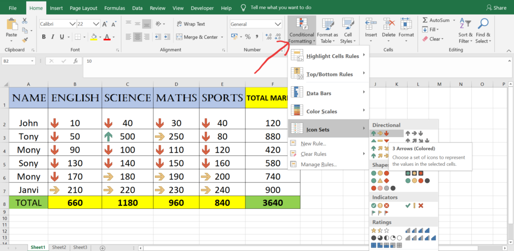
ICON SETS In Conditional Formatting ExcelHelp
Klik pada pilihan Conditional Formatting, pilih panel Top/Bottom Rules, dan kemudian pilih salah satu pilihan formatting yang ditunjukkan. Top/Bottom Rules dalam Excel. Di dalam kasus saya, saya akan memilih Above Average untuk menyoroti semua angka penjualan yang berada di atas rata-rata dalam set.